Anomaly Detection
Text Anomaly Detection focuses on analyzing words in log data, searching for anomalies. For each stream of logs algorithm will store statistical model containing calculated probability of word occurrence. Each source produce different type of log typical for the vendor. Using statistical approach we can easily identify uncommon entries and detect suspicious behavior in logs. Trained models can be saved in Model Library and used in real time in Network Probe pipeline.
Options
Select Anomaly Detection - Text in the Select Method field and set the common fields described in Create Use Case. The method adds the following fields:
AI Model: Build New From Scratch trains a new model, Take From Model Library reuses a model saved in the Model Library.
Exclude Pattern & Words: words and regular expressions that cannot appear in the rare word list.
Skip numbers: omits standalone numbers from the analysis.
Sampling Rate and Sampled Log Count: the percentage of documents to use and the resulting number of documents.
Rareness Threshold: the share of logs below which a word counts as rare.
Create Alert: creates an alert rule for the detected anomalies.
Exclude Pattern & Words: Enter one word or regular expression per line; the Regular Expression Guide link opens a syntax reference. You can set this field only when the use case runs in Run Once mode and does not reuse a model from the Model Library.

Skip numbers: When selected, standalone numbers are ignored in the analysis. Each number can significantly boost false-positive ratio. The option is off by default.
Actual Log Count: Gives information about number of documents for the selected source and build time frame. If the number becomes huge, consider using sampling.
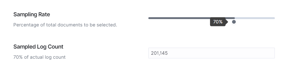
Sampling Rate: Set the percentage of documents to use, from 5% to 100% in steps of 5%. Sampled Log Count shows the resulting number of documents.
Rareness Threshold: A word counts as rare when it appears in less than the given percentage of logs. The shortcuts set values from 1-in-1K (0.1%) to 1-in-10M (0.00001%). The field is required.

Create Alert: When selected, saving the use case also creates an alert rule named AI <use case name> in the Empowered AI group. The rule fires for documents of this use case whose log anomaly score is higher than the value in the Anomaly Score field (100 by default). Deleting the use case does not delete this alert rule; delete it in Alerts > Alert Rules List.

Performance Tab for Text Anomaly Detection
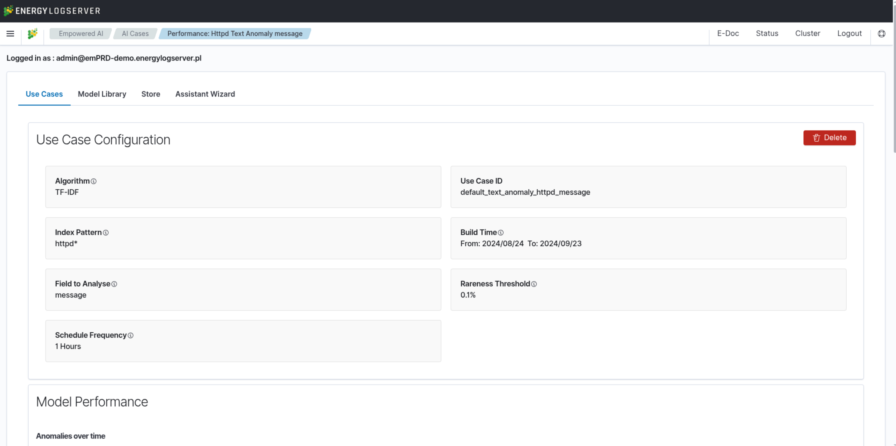
The Use Case Configuration section shows the settings of the use case, together with the Run and Delete buttons.
Understanding the Performance Graphs
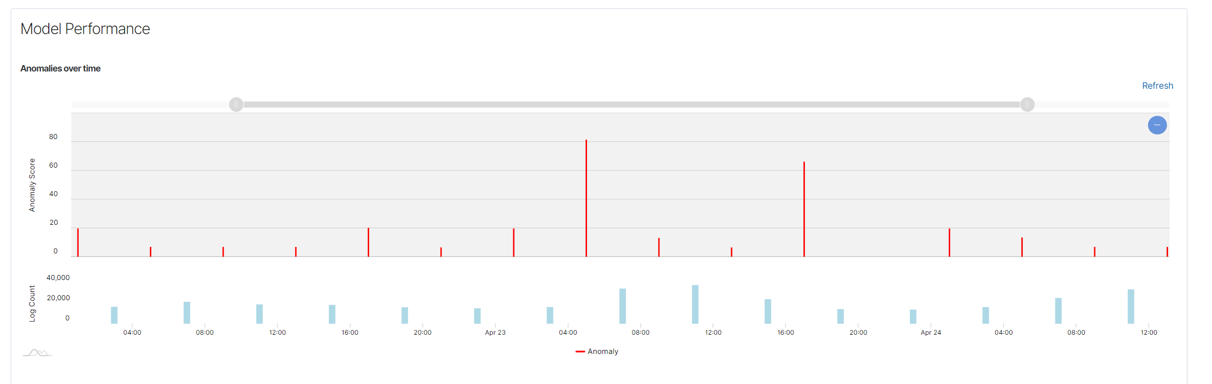
Anomalies over time: The red bars show the log anomaly score of each anomaly over time. The lower Log Count panel shows the number of logs per hour. Drag the slider handles above the chart to zoom in on a period.
Spread of Anomalies: Shows the distribution of anomaly scores from 0 to 100. Each dot represents the score of one anomalous log. Drag the slider handles to limit the table below to a score range.

Using the Performance Graphs
Monitoring Trends: Allows you to monitor trends and identify periods of abnormal activity.
Investigating Anomalies: By examining the anomaly markers, you can investigate the corresponding timestamps to understand the context.
Adjusting Parameters: If too many or too few anomalies are detected, consider adjusting the rareness threshold or sampling rate.
Anomaly Detection Table
At the bottom of the Performance tab, the Anomaly List tab lists the detected anomalies, sorted by log anomaly score in descending order.

Information in the Anomaly Detection Table:
Time Field: The time of the anomalous log. Click it to open the log in Discover.
Word anomaly score: The highest score among the rare words in the log.
Log anomaly score: The anomaly score for the entire log.
No. of rare words: The number of rare words detected in the log.
Rare words: The list of rare words detected in the log.
Text: A fragment of the text containing the detected anomalies.
Expanding a Row
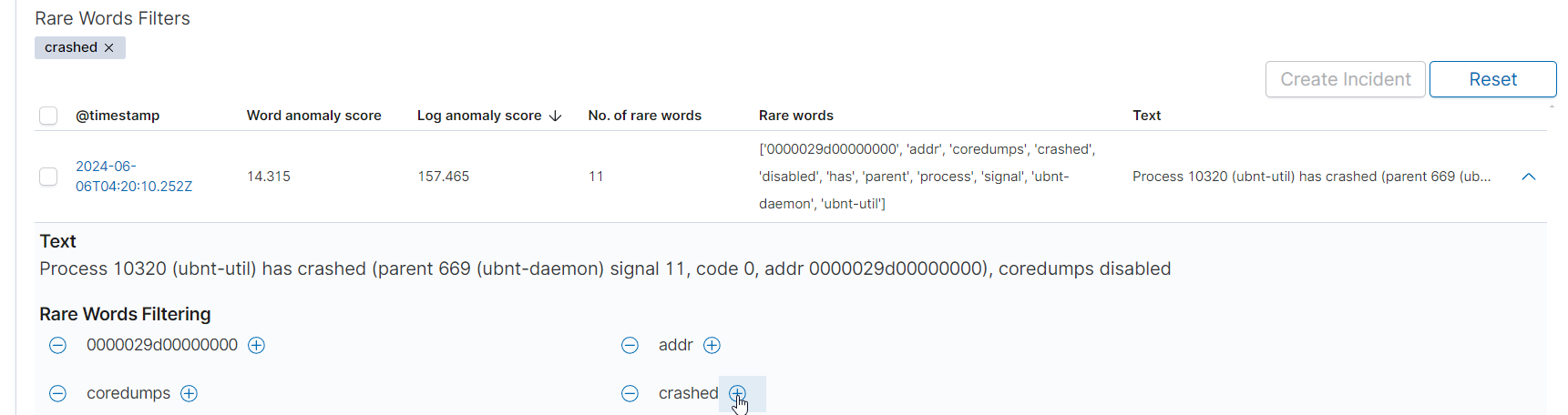
Click the arrow icon at the end of a row to expand it. The expanded row shows the full text of the log and the Rare Words Filtering list with every rare word found in it.
Filtering by Rare Words
In the Rare Words Filtering list of an expanded row, click + next to a word to show only the logs that contain it, or - to hide them. Each filter appears as a badge in the Rare Words Filters section at the top of the table. Click the badge to remove the filter.
Actions in the Table
Create Incident: Creates an incident for each selected row. The button is active when at least one row is selected.
Reset: Clears the row selection and the score range selected on the Spread of Anomalies chart. Rare word filters stay in place.
Distinct Anomaly List Table
The Distinct Anomaly List tab contains the same anomaly data as the first table but without duplicates. If the message is the same, it is displayed only once, and the Number of occurrences column shows how many times it was found. In the first table, all analyzed documents detected as anomalies are displayed, even if one document appears 200 times.
Univariate Anomaly Detection
Univariate Anomaly Detection identifies anomalies in a single number field. Select Anomaly Detection - Number in the Select Method field and leave the switch at Single value.
Step 1: Configuring the Univariate Anomaly Detection Rule
Field to Analyse: Select a numeric field, or select Take ‘log count’ itself as a signal to analyse to analyse the number of logs.
Multiply by Field: Optionally select a field; the use case builds a separate model for each value of this field.
Contamination Factor: The approximate percentage of data considered anomalous. The suggested value is between 0.5% and 3% (for example,
0.5%).Data Aggregation: Select the aggregation interval to be used for training the model. Available intervals are 30 minutes, 1 hour, 2 hours, 4 hours, 8 hours, 12 hours, and 1 day.

Complete the configuration of other settings, such as Start Date, Build Time Frame, and Scheduler options. These settings are described in Create Use Case.
Step 2: Running the Univariate Rule
Click Save & Run to start the anomaly detection immediately, or click Save and start the use case later with the play icon in the Use Cases list.
Performance Tab for Univariate Anomaly Detection
The Performance Tab provides a visual representation of the model’s performance, particularly focusing on the detected anomalies in a single data column over time.
Understanding the Performance Graph
The performance graph displays the aggregated values of the analysed field and highlights detected anomalies. The x-axis represents the timeline, while the y-axis shows the values of the analysed field, or Doc Count when the use case analyses the log count.

Key Elements of the Performance Graph
Actual (blue area)
The blue area represents the actual values of the monitored data over time. It helps in visualizing the normal behavior of the data and identifying patterns or trends.
Anomaly (red lines)
Red vertical lines mark the points where anomalies have been detected, showing the specific times when the data deviated from the normal pattern.
Drag the slider handles above the chart to zoom in on a period.
Interpreting the Graph
Spikes and Drops: Significant spikes or drops in the blue area could indicate unusual activity or anomalies in the data. Red lines on these spikes or drops confirm the detection of anomalies by the model.
Consistency: Consistent patterns without red lines suggest stable data behavior with no detected anomalies.
List of Anomalies
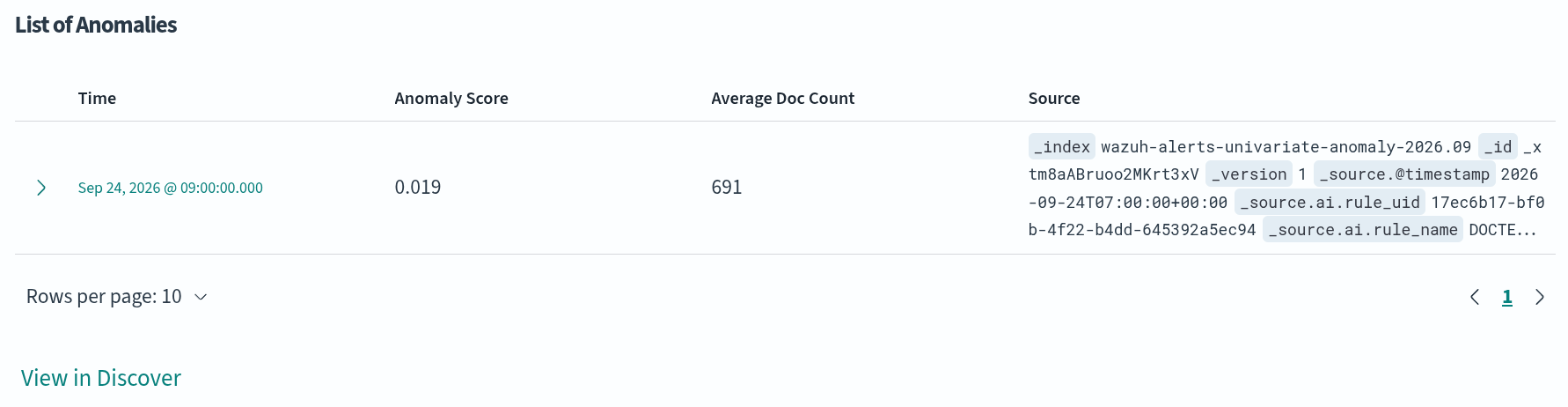
Below the chart, the List of Anomalies table lists the detected anomalies with the following columns:
Time: The start of the aggregation interval in which the anomaly was detected.
Anomaly Score: The score of the anomaly.
The aggregated value of the analysed field, for example Average Doc Count.
Source: The result document stored by the use case.
Click View in Discover to open the results in Discover.
Using the Performance Graph
Monitoring Trends: The graph allows you to monitor trends and identify periods of abnormal activity.
Investigating Anomalies: By examining the red lines, you can investigate the corresponding timestamps to understand the context of the anomalies.
Adjusting Parameters: If too many or too few anomalies are detected, consider adjusting the contamination factor or other model parameters to improve detection accuracy.
Multivariate Anomaly Detection
Multivariate Anomaly Detection identifies anomalies across multiple data columns. Below is a guide on configuring this use case.
Step 1: Configuring the Multivariate Anomaly Detection Rule
Choose Between Analyzing Single and Multiple Signals
Multi Values: Select Anomaly Detection - Number in the Select Method field and turn the switch to Multi values. Then select several numeric fields in Field to Analyse; the use case analyses them together.

Contamination Factor: The approximate percentage of data considered anomalous. The suggested value is between 0.5% and 3% (for example,
0.5%).Complete the configuration of other settings, such as Start Date, Build Time Frame, and Scheduler options. These settings are described in Create Use Case.
Step 2: Running the Multivariate Rule
Click Save & Run to start the anomaly detection immediately, or click Save and start the use case later with the play icon in the Use Cases list.
Performance Tab for Multivariate Anomaly Detection
The Performance Tab provides comprehensive visualizations and detailed information on detected anomalies over time. When the use case uses Multiply by Field, select the field value at the top of the page to see its results.
Visualizing Anomalies Over Time
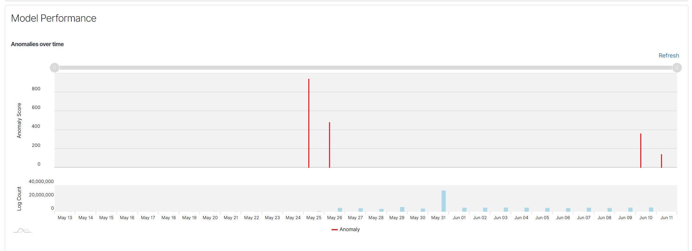
Anomalies over time: The X-axis represents time, while the Y-axis represents the anomaly score. Each red vertical line indicates an anomaly detected by the model at a specific time. The lower Log Count panel shows the number of logs. This visualization helps in identifying periods of high anomaly activity.
Spread of Anomalies: Shows the distribution of anomaly scores across the entire dataset. Each dot represents an anomaly score, and this chart helps to understand the spread and severity of anomalies in the data.
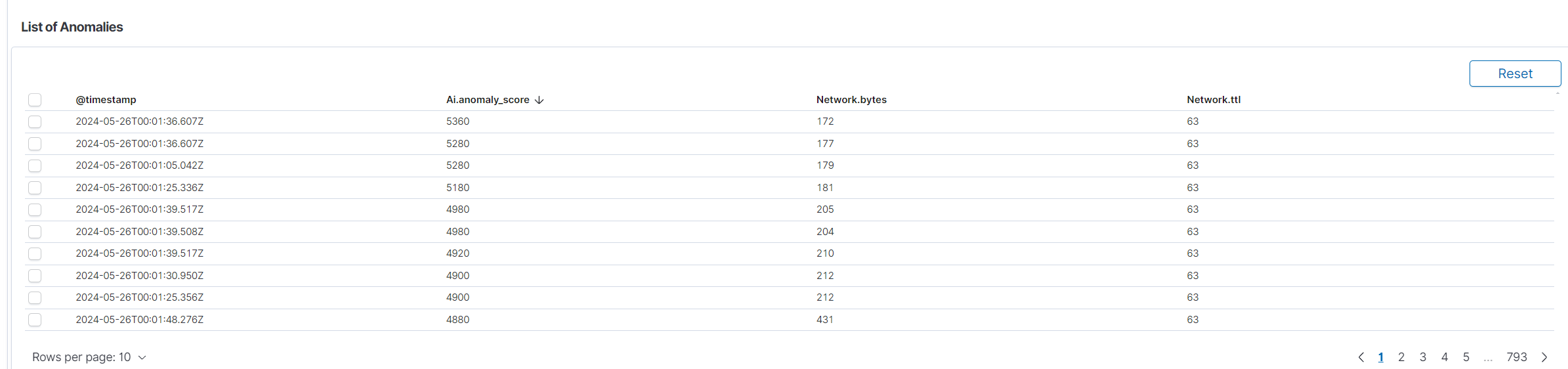
List of Anomalies: Below the charts, a table lists the values of the analysed fields for each anomaly. The columns are the analysed fields. Reset clears the selection, View in Discover opens the results in Discover, and Save Model saves the trained model in the Model Library.